Gridded data

Here, we develop a neural estimator for a spatial Gaussian process model with exponential covariance function and unknown range parameter  . The spatial domain is the unit square, data are simulated on a regular   grid (  locations), and we adopt the prior  .

Package dependencies

using NeuralEstimators
using Flux
using CairoMakie
using Distances
using Folds             # parallel simulation (start Julia with --threads=auto)
using LinearAlgebra     # Cholesky factorisation
using MLUtils: flatten

To improve computational efficiency, various GPU backends are supported. Once the relevant package is loaded and a compatible GPU is available, it will be used automatically:

NVIDIA GPUs

using CUDA, cuDNN

AMD ROCm GPUs

using AMDGPU

Metal M-Series GPUs

using Metal

Intel GPUs

using oneAPI

Sampling parameters

Simulation from Gaussian processes requires computing the Cholesky factor of a covariance matrix, which is expensive but reusable across repeated simulations from the same parameters. We therefore define a custom type Parameters subtyping AbstractParameterSet to store both the parameters and their corresponding Cholesky factors:

struct Parameters <: AbstractParameterSet
	θ
	L
end

We define two constructors: one that accepts an integer and samples from the prior (used during training), and one that accepts a parameter matrix directly (useful for parametric bootstrap at inference time):

function sampler(K::Integer)
    θ = 0.5 * rand(K)               # K samples from p(θ) = Unif(0, 0.5)
    Parameters(NamedMatrix(θ = θ))  # Wrap as a named matrix and pass to matrix constructor
end

function Parameters(θ::AbstractMatrix; grid_dim = 16)
	# Spatial locations: regular grid over the unit square
	pts = range(0, 1, length = grid_dim)
	S = expandgrid(pts, pts)

	# Pairwise distances, covariance matrices, and Cholesky factors
	D = pairwise(Euclidean(), S, dims = 1)
	K = size(θ, 2)
	L = Folds.map(1:K) do k
		Σ = exp.(-D ./ θ[k])
		cholesky(Symmetric(Σ)).L
	end

	Parameters(θ, L)
end

Simulating data

We store each simulated data set as a four-dimensional array of dimension    , where the third dimension is the number of channels (singleton for a univariate process) and the fourth stores independent replicates:

function simulator(parameters::Parameters)
	Z = Folds.map(parameters.L) do L
		n = size(L, 1)
		z = L * randn(n, 1)
		grid_dim = isqrt(n)   # NB assumes a square grid
		reshape(z, grid_dim, grid_dim, 1)
	end
	stack(Z)
end

Constructing the neural network

For data collected over a regular grid, the neural network is typically a convolutional neural network (CNN; see, e.g., Dumoulin and Visin, 2016). A simple CNN that could be used in the current example is:

d = 1                # dimension of the parameter vector θ
num_summaries = 3d   # number of summary statistics for θ

network = Chain(
	Conv((3, 3), 1 => 32, gelu),    # 3×3 filter, 1 → 32 channels
	MaxPool((2, 2)),                # 2×2 max pooling
	Conv((3, 3), 32 => 64, gelu),   # 3×3 filter, 32 → 64 channels
	GlobalMeanPool(),               # collapse spatial dimensions
	flatten,                        # flatten for dense layers
	Dense(64, 64, gelu), 
	Dense(64, 64, gelu), 
	Dense(64, num_summaries)
)

The inclusion of a global pooling layer (e.g., GlobalMeanPool) allows the network to accommodate grids of varying dimensions. However, standard CNNs require a fixed input size during training due to their rigid input structure. To handle varying grid sizes during training, use a DeepSet as described in Bonus: Replicated data.

In practice, deeper architectures with residual connections (see ResidualBlock) often lead to improved performance. For example:

network = Chain(
	Conv((3, 3), 1 => 16, pad=1, bias=false), 
	BatchNorm(16, relu),   
	ResidualBlock((3, 3), 16 => 16),                               
	ResidualBlock((3, 3), 16 => 32, stride=2),                     
	ResidualBlock((3, 3), 32 => 64, stride=2),                     
	ResidualBlock((3, 3), 64 => 128, stride=2),                    
	GlobalMeanPool(),                                              
	flatten,
	Dense(128, 64, gelu), 
	Dense(64, 64, gelu), 
	Dense(64, num_summaries)
)

Constructing the neural estimator

We now construct a NeuralEstimator by wrapping the neural network in the subtype corresponding to the intended inferential method:

Point estimator

estimator = PointEstimator(network, d; num_summaries = num_summaries)

Posterior estimator

estimator = PosteriorEstimator(network, d; num_summaries = num_summaries)

Ratio estimator

estimator = RatioEstimator(network, d; num_summaries = num_summaries)

Training the estimator

We train the estimators using fixed parameter instances to avoid repeated Cholesky factorisations (see Storing expensive intermediate objects for data simulation and On-the-fly and just-in-time simulation for further discussion):

K = 5000
θ_train = sampler(K)
θ_val   = sampler(K)
estimator = train(estimator, θ_train, θ_val, simulator)

The empirical risk (average loss) over the training and validation sets can be plotted using plotrisk. One may wish to save a trained estimator and load it in a later session: see Saving and loading estimators for details on how this can be done.

Assessing the estimator

The function assess can be used to assess the trained estimator:

θ_test = sampler(1000)  
Z_test = simulator(θ_test)
assessment = assess(estimator, θ_test, Z_test)

The resulting Assessment object contains ground-truth parameters, estimates, and other quantities that can be used to compute quantitative and qualitative diagnostics:

bias(assessment)
rmse(assessment)
plot(assessment)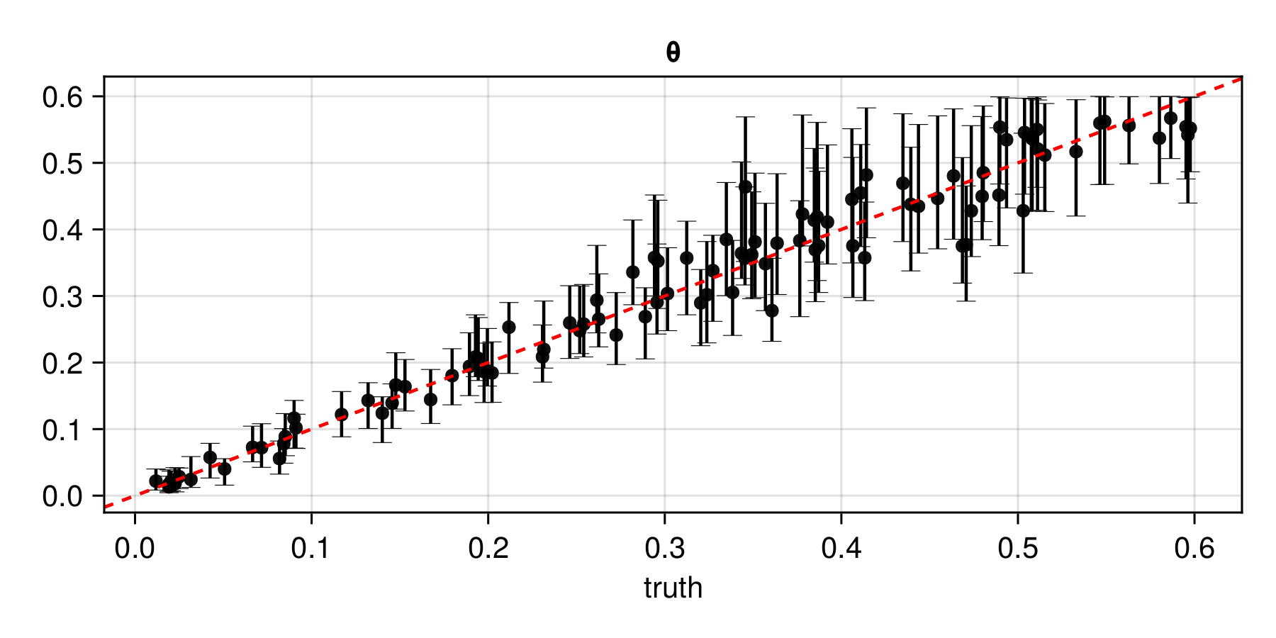

Applying the estimator to observed data

Once an estimator is deemed to be well calibrated, it may be applied to observed data (below, we use simulated data as a stand-in for observed data):

θ = Parameters(Matrix([0.1]'))   # ground truth (not known in practice)
Z = simulator(θ)                 # stand-in for real data

Point estimator

estimate(estimator, Z)             # point estimate

Posterior estimator

sampleposterior(estimator, Z)      # posterior sample

Ratio estimator

sampleposterior(estimator, Z)      # posterior sample

Bonus: Incomplete data

In practice, data are often incomplete, for example, due to cloud cover or limitations in remote-sensing instruments. Missing data can be handled using the missing-data methods implemented in the package, in particular via masking or the Monte Carlo EM algorithm.

Bonus: Replicated data

Parameter estimation from replicated data is commonly required in statistical applications. For example, it arises when fitting classical geostatistical models with time replicates treated as independent, and in the analysis of spatial extremes.

To fit our spatial Gaussian process model with replicates, we modify the simulator as follows:

function simulator(parameters::Parameters, m)
	Folds.map(parameters.L) do L
		n = size(L, 1)
		z = L * randn(n, m)
		grid_dim = isqrt(n)   # NB assumes a square grid
		reshape(z, grid_dim, grid_dim, 1, m)
	end
end

A flexible framework for handling replicated data is DeepSets, implemented in the package via DeepSet.

A DeepSet consists of three components: an inner network that acts directly on each data replicate; an aggregation function that combines the resulting representation; and an outer network (typically an MLP) that maps the aggregated features to the output space (here, a space of summary statistics). The architecture of the inner network depends on the structure of the data; for gridded data, we use a CNN.

d = 1                # dimension of the parameter vector θ
num_summaries = 3d   # number of summary statistics for θ

# Inner network (CNN, almost identical to that given above)
ψ = Chain(
	Conv((3, 3), 1 => 32, gelu),
	MaxPool((2, 2)),
	Conv((3, 3), 32 => 64, gelu),
	GlobalMeanPool(),
	flatten,
	Dense(64, 64, gelu), 
	Dense(64, 64, gelu), 
	Dense(64, 64)
)

# Outer network (MLP)
ϕ = Chain(
	Dense(64, 64, relu), 
	Dense(64, num_summaries)
)

# DeepSet object
network = DeepSet(ψ, ϕ)

An additional advantage of using a DeepSet is that the input structure is more flexible than that of a generic CNN. In particular, it operates on a vector of arrays, where each array corresponds to a single data set and may have arbitrary dimension

The rest of the code given above remains exactly the same, with the number of replicates passed into train via the keyword argument simulator_args:

Point estimator

estimator = PointEstimator(network, d; num_summaries = num_summaries)

Posterior estimator

estimator = PosteriorEstimator(network, d; num_summaries = num_summaries)

Ratio estimator

estimator = RatioEstimator(network, d; num_summaries = num_summaries)

estimator = train(estimator, θ_train, θ_val, simulator; simulator_args = 10)

A key advantage of the DeepSet representation is that it can be applied to data sets of arbitrary sample size . However, the posterior distribution, and summaries derived from it, typically depends on . If data sets with varying are envisaged, the estimator should be designed to account for this dependence. See Variable sample sizes for further details.