Spatio-temporal Data

Here, we develop a neural estimator for data modelled as a Spatio-Temporal Gaussian Random Field (GRF). This model can be used for environmental phenomena such as sea surface temperature (SST) that exhibit correlation across both space and time.

We assume that the data are observed at locations on a regular spatial grid over time steps. Let   denote the vector of observations at time  . The data are modelled as correlated mean-zero Gaussian random variables with a separable spatio-temporal covariance function given by the product of a Matérn spatial covariance function and an AR(1) temporal covariance function:

where    denotes the Matérn covariance function with smoothness parameter fixed to , and   and   are parameters controlling the strength of spatial and temporal dependence, respectively. This model can be equivalently expressed as the dynamic system

where    ,  , and    .

We place independent uniform priors on the parameters:   and  .

Package dependencies

using NeuralEstimators
using NeuralEstimators: getobs, numobs
using Flux
using Folds                    # parallel simulation (start Julia with --threads=auto)
using Distances
using Distributions: Uniform
using LinearAlgebra
using Statistics
using CairoMakie

This example uses convolutional neural networks (CNNs), which are computationally intensive but highly parallelisable and therefore greatly benefit from GPU acceleration. Various GPU backends are supported and, once the relevant package is loaded and a compatible GPU is available, it will be used automatically:

NVIDIA GPUs

using CUDA, cuDNN

AMD ROCm GPUs

using AMDGPU

Metal M-Series GPUs

using Metal

Intel GPUs

using oneAPI

Sampling parameters

We first define a function to sample parameters from the prior distribution. Here, we store the parameters as a NamedMatrix so that parameter estimates are automatically labelled, though this is not required:

function sampler(K)
    NamedMatrix(
        θ₁ = rand(Uniform(0.05, 0.5), K),
        θ₂ = rand(Uniform(0.1, 0.9), K)
    )
end

Simulating data and constructing the neural network

The simulator and the neural network are designed in tandem: the architecture is chosen based on the structure of the data, and the simulator must return data in a format appropriate for the chosen architecture.

The data are spatio-temporally dependent and observed over a regular spatio-temporal grid. Several architectures could handle these data correctly:

• CNN with channel dimensions: treats each time step as a channel. Simple and effective but requires fixed .

• CNN + RNN/LSTM/Transformer: a CNN extracts spatial features from each time slice, and an RNN/LSTM/Transformer processes them sequentially to capture temporal dependence. Handles variable naturally but more computationally expensive.

• DeepSet with CNN inner network: for an AR(1) process, the first differences    are exchangeable, so a DeepSet with a CNN inner network applied to each difference field can be used. Handles variable naturally and computationally efficiently.

We adopt the last approach, as it is simple to implement, exploits the model structure, and is computationally efficient.

DeepSet objects act on vectors, where each element of the vector is associated with one parameter vector , and where the format of each element depends on the chosen architecture for the inner network. In our example, the inner network is a CNN acting on data collected over a two-dimensional spatial grid, so each element of the vector should be stored as a 4-dimensional array of shape , with the time slices stored in the 4ᵗʰ (batch) dimension. Here, for simplicity, we return the first differences rather than the raw data for immediate input to the neural network.

# Matérn covariance with unknown range parameter and fixed smoothness parameter 3/2 
function matern15(d, ρ)
    d == 0.0 && return 1.0
    r = sqrt(3) * d / ρ
    return (1 + r) * exp(-r)
end

# Compute Δₜ for t = 2, ..., T
function firstdifference(Z)
    # Equivalently: Z[:, :, :, 2:end] - Z[:, :, :, 1:end-1]
    getobs(Z, 2:numobs(Z)) - getobs(Z, 1:numobs(Z)-1)
end

# Simulate a single spatio-temporal field with T time steps
function simulator(θ::AbstractVector, T::Integer; grid_size = 10)
    ρ = θ["θ₁"]
    φ = θ["θ₂"]

    # Regular spatial grid
    locs = [(i/grid_size, j/grid_size) for i in 1:grid_size for j in 1:grid_size]
    n_spatial = length(locs)

    # Spatial covariance matrix and its Cholesky factor
    Σ = [matern15(norm(collect(locs[i]) .- collect(locs[j])), ρ) for i in 1:n_spatial, j in 1:n_spatial]
    L = cholesky(Σ + 1e-6 * I).L

    # Dynamic system
    Z = zeros(n_spatial, T)
    Z[:, 1] = L * randn(n_spatial)
    for t in 2:T
        Z[:, t] = φ .* Z[:, t-1] .+ sqrt(1 - φ^2) .* (L * randn(n_spatial))
    end

    # Reshape into format required by our chosen architecture
    Z = reshape(Z, grid_size, grid_size, 1, T)
    return firstdifference(Z)
end
simulator(θ::AbstractVector, T)         = simulator(θ, rand(T))
simulator(θ::AbstractMatrix, T = 10:30) = Folds.map(ϑ -> simulator(ϑ, T), eachcol(θ))

With this data format, the DeepSet inner network ψ processes each difference field independently, and the outer network ϕ maps the aggregated latent features to summary statistics:

d  = 2     # number of parameters
w  = 128   # hidden layer width
nc = 32    # channels in final conv layer and dimension of DeepSet latent space 
num_summaries  = 3d  # number of summaries output by the network

ψ = Chain(
    Conv((3, 3), 1 => 16, relu; pad = 1),
    MaxPool((2, 2)),
    Conv((3, 3), 16 => nc, relu; pad = 1),
    GlobalMeanPool(),
    Flux.flatten,
)
ϕ = Chain(
    Dense(nc, w, relu),
    Dense(w, w, relu),
    Dense(w, w, relu),
    Dense(w, num_summaries),
)
network = DeepSet(ψ, ϕ)

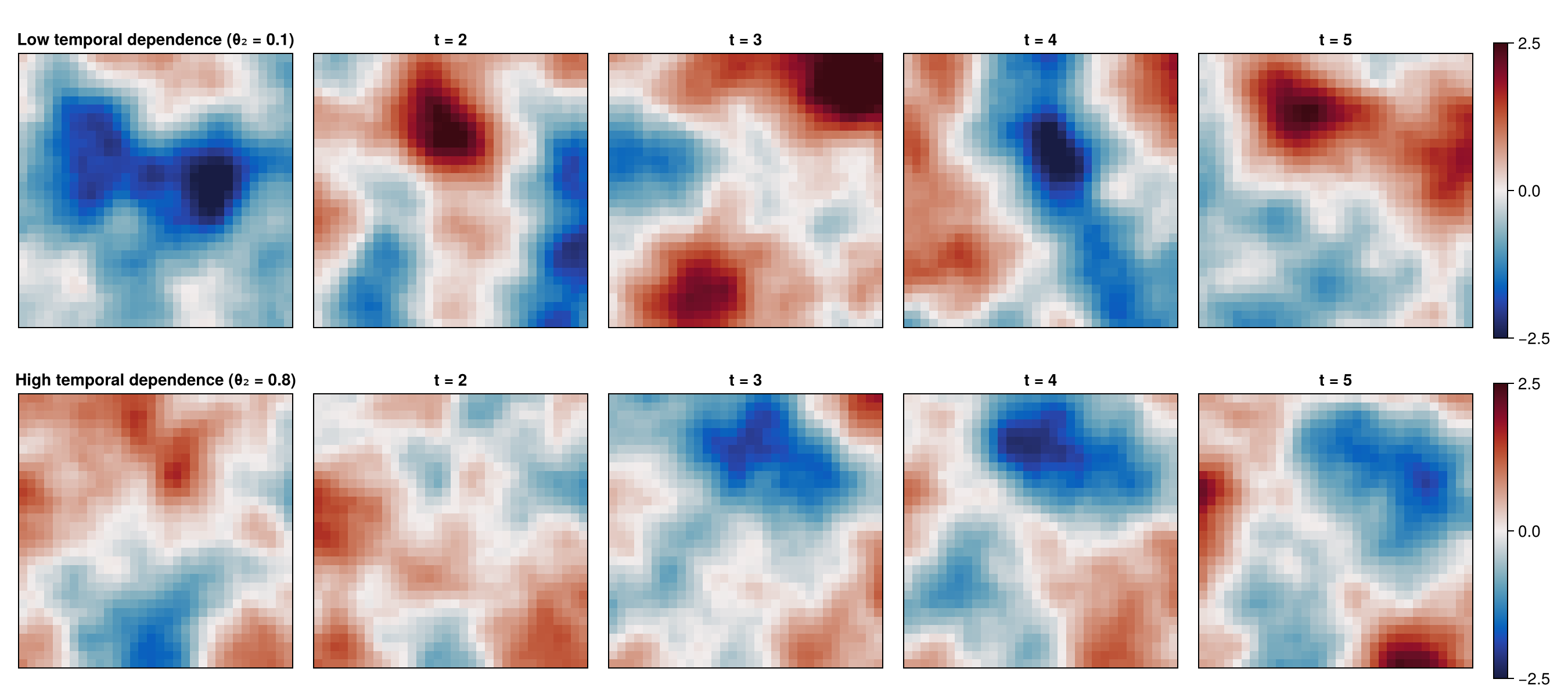
Constructing the neural estimator

We now construct a NeuralEstimator by wrapping the neural network in the subtype corresponding to the intended inferential method:

Point estimator

estimator = PointEstimator(network, d; num_summaries = num_summaries)

Posterior estimator

estimator = PosteriorEstimator(network, d; num_summaries = num_summaries)

Ratio estimator

estimator = RatioEstimator(network, d; num_summaries = num_summaries)

Training the estimator

Next, we train the estimator using train. One may pass sampler and simulator directly to train for on-the-fly simulation, but here we pre-simulate fixed training sets, which can be faster when the simulator is expensive:

K = 2500 # size of the training set
θ_train = sampler(K)
θ_val   = sampler(K)
Z_train = simulator(θ_train);
Z_val   = simulator(θ_val);
estimator = train(estimator, θ_train, θ_val, Z_train, Z_val)

# Alternatively, simulate on-the-fly:
# estimator = train(estimator, sampler, simulator; K = K)

The empirical risk (average loss) over the training and validation sets can be plotted using plotrisk.

One may wish to save a trained estimator and load it in a later session: see Saving and loading neural estimators for details on how this can be done.

Assessing the estimator

The function assess can be used to assess the trained estimator:

θ_test = sampler(1000)
Z_test = simulator(θ_test, 20);
assessment = assess(estimator, θ_test, Z_test)

The resulting Assessment object contains ground-truth parameters, estimates, and other quantities that can be used to compute quantitative and qualitative diagnostics:

bias(assessment)    # θ₁ = ..., θ₂ = ...
rmse(assessment)    # θ₁ = ..., θ₂ = ...
plot(assessment)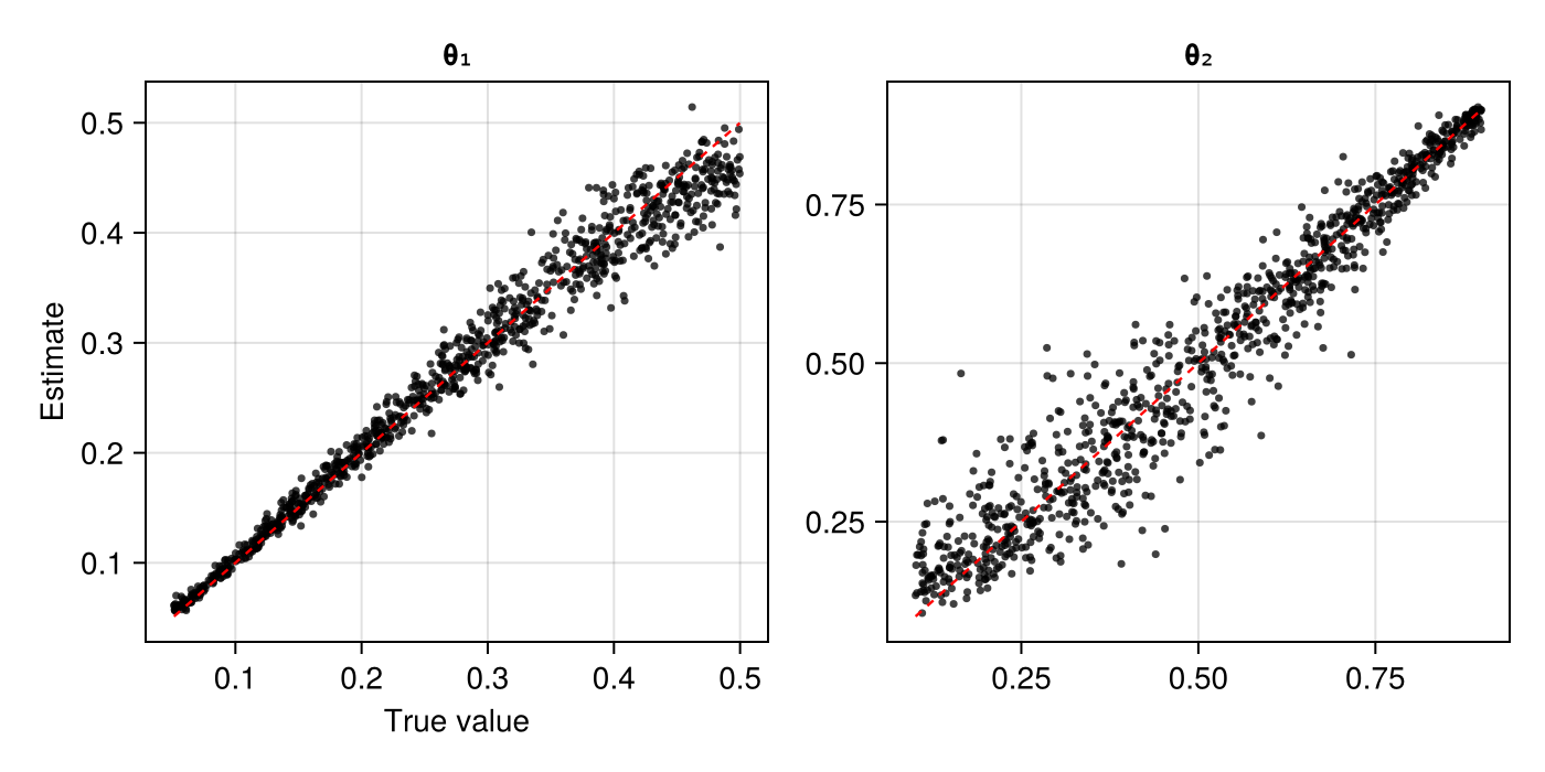

Applying the estimator to observed data

Once an estimator is deemed to be well calibrated, it may be applied to observed data (below, we use simulated data as a stand-in for observed data):

θ = sampler(1)
Z = simulator(θ, 20);

Point estimator

estimate(estimator, Z)

Posterior estimator

sampleposterior(estimator, Z)

Ratio estimator

sampleposterior(estimator, Z)