Replicated unstructured data

Here, we develop a neural estimator to infer   from data  , where   . We adopt the marginal priors   and  .

Package dependencies

using NeuralEstimators
using Flux             
using Distributions: InverseGamma
using CairoMakie

To improve computational efficiency, various GPU backends are supported. Once the relevant package is loaded and a compatible GPU is available, it will be used automatically:

NVIDIA GPUs

using CUDA

AMD ROCm GPUs

using AMDGPU

Metal M-Series GPUs

using Metal

Intel GPUs

using oneAPI

Sampling parameters

We first define a function to sample parameters from the prior distribution. Here, we store the parameters as a NamedMatrix so that parameter estimates are automatically labelled, though this is not required:

function sampler(K)
	NamedMatrix(
		μ = randn(K), 
		σ = rand(InverseGamma(3, 1), K)
	)
end

Simulating data

Next, we define the statistical model implicitly through simulation. Our data consist of independent replicates, and we wish to accommodate varying across data sets. We therefore use a DeepSets architecture, where the simulated data for each parameter vector are stored as a separate element of a Vector. In this example each replicate is univariate, so each element is a Matrix with one row and columns.

We define three methods for simulating data, illustrating Julia's multiple dispatch and short-form function syntax: the first simulates a data set of fixed size for a single parameter vector; the second simulates a data set of random size drawn from a range; and the third applies these over a matrix of parameter vectors:

simulator(θ::AbstractVector, m::Integer) = θ["μ"] .+ θ["σ"] .* randn(1, m)
simulator(θ::AbstractVector, m) = simulator(θ, rand(m))
simulator(θ::AbstractMatrix, m = 10:100) = [simulator(ϑ, m) for ϑ in eachcol(θ)]

Constructing the neural network

In this package, the neural network specified by the user is typically a summary network that transforms data into a vector of summary statistics for , where is user-specified. A common heuristic is to set to a multiple of , the number of unknown parameters (e.g.,  ).

In this example, our data are replicated, and we therefore adopt the DeepSets framework, implemented via DeepSet. A DeepSet consists of three components: an inner network that acts directly on each data replicate; a function that aggregates the outputs of the inner network; and an outer network (typically an MLP) that maps the aggregated output to . The architecture of the inner network depends on the structure of the data; for unstructured data (i.e., without spatial or temporal correlation within each replicate), an MLP is used, with input dimension matching the dimensionality of each replicate (here, one).

n = 1                # dimension of each data replicate (univariate)
d = 2                # dimension of the parameter vector θ
num_summaries = 3d   # number of summary statistics for θ
w = 64               # width of each hidden layer

ψ = Chain(Dense(n, w, relu), Dense(w, w, relu))         # inner network
ϕ = Chain(Dense(w, w, relu), Dense(w, num_summaries))   # outer network
network = DeepSet(ψ, ϕ)

Constructing the neural estimator

We now construct a NeuralEstimator by wrapping the neural network in the subtype corresponding to the intended inferential method:

Point estimator

estimator = PointEstimator(network, d; num_summaries = num_summaries)

Posterior estimator

estimator = PosteriorEstimator(network, d; num_summaries = num_summaries)

Ratio estimator

estimator = RatioEstimator(network, d; num_summaries = num_summaries)

Training the estimator

Next, we train the estimator using train. Below, we pass our user-defined functions for sampling parameters and simulating data, but one may also pass fixed parameter and/or data instances:

estimator = train(estimator, sampler, simulator)

The empirical risk (average loss) over the training and validation sets can be plotted using plotrisk.

One may wish to save a trained estimator and load it in a later session: see Saving and loading neural estimators for details on how this can be done.

Assessing the estimator

The function assess can be used to assess the trained estimator:

θ_test = sampler(1000)           # test parameters
Z_test = simulator(θ_test, 50)   # test data, with 50 replicates in each data set
assessment = assess(estimator, θ_test, Z_test)

The resulting Assessment object contains ground-truth parameters, estimates, and other quantities that can be used to compute quantitative and qualitative diagnostics:

bias(assessment)      # μ = 0.002, σ = 0.017
rmse(assessment)      # μ = 0.086, σ = 0.078
risk(assessment)      # 0.055
plot(assessment)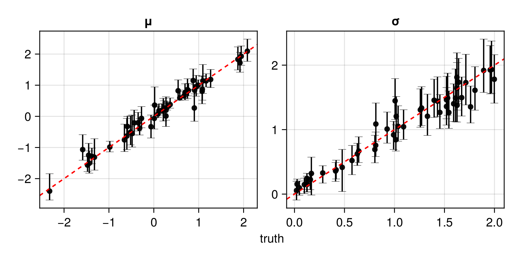

Applying the estimator to observed data

Once an estimator is deemed to be well calibrated, it may be applied to observed data (below, we use simulated data as a stand-in for observed data):

θ = sampler(1)                      # ground truth (not known in practice)
Z = simulator(θ, 100)               # stand-in for real data

Point estimator

estimate(estimator, Z)             # point estimate
interval(bootstrap(estimator, Z))  # 95% non-parametric bootstrap intervals

Posterior estimator

sampleposterior(estimator, Z)      # posterior sample

Ratio estimator

sampleposterior(estimator, Z)      # posterior sample