Missing or censored data

Missing data

Neural networks do not naturally handle missing data, and this property can preclude their use in a broad range of applications. Here, we describe two techniques that alleviate this challenge in the context of parameter point estimation: the masking approach and the expectation-maximisation (EM) approach.

As a running example, we consider a Gaussian process model where the data are collected over a regular grid, but where some elements of the grid are unobserved. This situation often arises in, for example, remote-sensing applications, where the presence of cloud cover prevents measurement in some places. Below, we load the packages needed in this example, and define some aspects of the model that will remain constant throughout (e.g., the prior, the spatial domain). We also define types and functions for sampling from the prior distribution and for simulating marginally from the data model.

using NeuralEstimators, Flux
using Distributions: Uniform
using Distances, LinearAlgebra
using MLUtils: flatten
using SpecialFunctions: besselk, gamma
using Statistics: mean

# Prior and dimension of parameter vector
Π = (τ = Uniform(0, 1.0), ρ = Uniform(0, 0.4))
d = length(Π)

# Define the grid and compute the distance matrix
points = range(0, 1, 16)
S = expandgrid(points, points)
D = pairwise(Euclidean(), S, dims = 1)

# Collect model information for later use
ξ = (Π = Π, S = S, D = D)

# Struct for storing parameters and Cholesky factors
struct Parameters <: AbstractParameterSet
	θ
	L
end

# Matern covariance function
function matern(h, ρ, ν, σ² = one(typeof(h)))

    @assert h >= 0 "h should be non-negative"
    @assert ρ > 0 "ρ should be positive"
    @assert ν > 0 "ν should be positive"

    if h == 0
        σ²
    else
        d = h / ρ
        σ² * ((2^(1 - ν)) / gamma(ν)) * d^ν * besselk(ν, d)
    end
end

# Constructor for above struct
function sample(K::Integer, ξ)

	# Sample parameters from the prior
	Π = ξ.Π
	τ = rand(Π.τ, K)
	ρ = rand(Π.ρ, K)
	ν = 1 # fixed smoothness

	# Compute Cholesky factors
	L = map(1:K) do k
		C = matern.(UpperTriangular(ξ.D), ρ[k], ν, 1)
		L = cholesky(Symmetric(C)).L
		convert(Array, L)
	end
	L = Base.stack(L)

	# Concatenate into matrix
	θ = permutedims(hcat(τ, ρ))

	Parameters(θ, L)
end

# Marginal simulation from the data model
function simulate(parameters::Parameters, m::Integer)

	K = size(parameters, 2)
	τ = parameters.θ[1, :]
	L = parameters.L
	G = isqrt(size(L, 1)) # side-length of grid

	Z = map(1:K) do k
		z = simulategaussian(L[:, :, k], m)
		z = z + τ[k] * randn(size(z)...)
		z = reshape(z, G, G, 1, :)
		z
	end

	return Z
end

The masking approach

The first missing-data technique that we consider is the so-called masking approach of Wang et al. (2024); see also the discussion by Sainsbury-Dale et al. (2025, Sec. 2.2). The strategy involves completing the data by replacing missing values with zeros, and using auxiliary variables to encode the missingness pattern, which are also passed into the network.

Let denote the complete-data vector. Then, the masking approach considers inference based on , a vector of indicator variables that encode the missingness pattern (with elements equal to one or zero if the corresponding element of is observed or missing, respectively), and

where denotes elementwise multiplication and the product of a missing element and zero is defined to be zero. Irrespective of the missingness pattern, and have the same fixed dimensions and hence may be processed easily using a single neural network. A neural estimator is then trained on realisations of which, by construction, do not contain any missing elements.

The manner in which and are combined depends on the multivariate structure of the data and the chosen architecture. For example, when the data are gridded and the neural network is a CNN, then and can be concatenated along the channels dimension (i.e., the penultimate dimension of the array). The construction of augmented data sets from incomplete data is facilitated by the helper function encodedata().

Since the missingness pattern is now an input to the neural network, it must be incorporated during the training phase. When interest lies only in making inference from a single already-observed data set, is fixed and known, and the Bayes risk remains unchanged. However, amortised inference, whereby one trains a single neural network that will be used to make inference with many data sets, requires a joint model for the data and the missingness pattern , which is here defined as follows (see the helper function removedata()):

# Marginal simulation from the data model and a MCAR missingness model
function simulatemissing(parameters::Parameters, m::Integer)

	Z = simulate(parameters, m)   # complete data

	UW = map(Z) do z
		prop = rand()             # sample a missingness proportion
		z = removedata(z, prop)   # randomly remove a proportion of the data
		uw = encodedata(z)        # replace missing entries with zero and encode missingness pattern
		uw
	end

	return UW
end

Next, we construct and train a masked neural Bayes estimator using a CNN architecture. Here, the first convolutional layer takes two input channels, since we store the augmented data in the first channel and the missingness pattern in the second. We construct a point estimator, but the masking approach is applicable with any other kind of estimator (see Estimators):

# Construct DeepSet object
ψ = Chain(
	Conv((10, 10), 2 => 16,  relu),
	Conv((5, 5),  16 => 32,  relu),
	Conv((3, 3),  32 => 64, relu),
	flatten
	)
ϕ = Chain(Dense(64, 256, relu), Dense(256, d, exp))
network = DeepSet(ψ, ϕ)

# Initialise point estimator
θ̂ = PointEstimator(network)

# Train the masked neural Bayes estimator
θ̂ = train(θ̂, sample, simulatemissing, simulator_args = 1, ξ = ξ, K = 1000, epochs = 10)

Once trained, we can apply our masked neural Bayes estimator to (incomplete) observed data. The data must be encoded in the same manner as during training. Below, we use simulated data as a surrogate for real data, with a missingness proportion of 0.25:

θ = sample(1, ξ)     # true parameters
Z = simulate(θ, 1)[1]    # complete data
Z = removedata(Z, 0.25)  # "observed" incomplete data (i.e., with missing values)
UW = encodedata(Z)       # augmented data {U, W}
θ̂(UW)                    # point estimate

The EM approach

Let and denote the observed and unobserved (i.e., missing) data, respectively, and let   denote the complete data. A classical approach to facilitating inference when data are missing is the expectation-maximisation (EM) algorithm. The neural EM algorithm (Sainsbury-Dale et al., 2025, Sec. 2.3) is an approximate version of the conventional (Bayesian) Monte Carlo EM algorithm which, at the th iteration, updates the parameter vector through

where realisations of the missing-data component,   , are sampled from the probability distribution of given and , and where   is a concentrated version of the original prior density. Given the conditionally simulated data, the neural EM algorithm performs the above EM update using a neural network that returns the MAP estimate (i.e., the posterior mode) using (complete) conditionally simulated data.

First, we construct a neural approximation of the MAP estimator. In this example, we will take  . When is taken to be reasonably large and the prior is uniform, one may lean on the Bernstein-von Mises theorem to train the neural Bayes estimator under linear or quadratic loss; otherwise, one should train the estimator under a continuous relaxation of the 0–1 loss (e.g., the tanhloss() in the limit  ). This is done as follows:

# Construct DeepSet object
ψ = Chain(
	Conv((10, 10), 1 => 16,  relu),
	Conv((5, 5),  16 => 32,  relu),
	Conv((3, 3),  32 => 64, relu),
	flatten
	)
ϕ = Chain(
	Dense(64, 256, relu),
	Dense(256, d, exp)
	)
network = DeepSet(ψ, ϕ)

# Initialise point estimator
θ̂ = PointEstimator(network)

# Train neural Bayes estimator
H = 50
θ̂ = train(θ̂, sample, simulate, simulator_args = H, ξ = ξ, K = 1000, epochs = 10)

Next, we define a function for conditional simulation (see EM for details on the required format of this function):

function simulateconditional(Z::M, θ; nsims::Integer = 1, ξ) where {M <: AbstractMatrix{Union{Missing, T}}} where T

	# Save the original dimensions
	dims = size(Z)

	# Convert to vector
	Z = vec(Z)

	# Compute the indices of the observed and missing data
	I₁ = findall(z -> !ismissing(z), Z) # indices of observed data
	I₂ = findall(z -> ismissing(z), Z)  # indices of missing data
	n₁ = length(I₁)
	n₂ = length(I₂)

	# Extract the observed data and drop Missing from the eltype of the container
	Z₁ = Z[I₁]
	Z₁ = [Z₁...]

	# Distance matrices needed for covariance matrices
	D   = ξ.D # distance matrix for all locations in the grid
	D₂₂ = D[I₂, I₂]
	D₁₁ = D[I₁, I₁]
	D₁₂ = D[I₁, I₂]

	# Extract the parameters from θ
	τ = θ[1]
	ρ = θ[2]

	# Compute covariance matrices
	ν = 1 # fixed smoothness
	Σ₂₂ = matern.(UpperTriangular(D₂₂), ρ, ν); Σ₂₂[diagind(Σ₂₂)] .+= τ^2
	Σ₁₁ = matern.(UpperTriangular(D₁₁), ρ, ν); Σ₁₁[diagind(Σ₁₁)] .+= τ^2
	Σ₁₂ = matern.(D₁₂, ρ, ν)

	# Compute the Cholesky factor of Σ₁₁ and solve the lower triangular system
	L₁₁ = cholesky(Symmetric(Σ₁₁)).L
	x = L₁₁ \ Σ₁₂

	# Conditional covariance matrix, cov(Z₂ ∣ Z₁, θ),  and its Cholesky factor
	Σ = Σ₂₂ - x'x
	L = cholesky(Symmetric(Σ)).L

	# Conditonal mean, E(Z₂ ∣ Z₁, θ)
	y = L₁₁ \ Z₁
	μ = x'y

	# Simulate from the distribution Z₂ ∣ Z₁, θ ∼ N(μ, Σ)
	z = randn(n₂, nsims)
	Z₂ = μ .+ L * z

	# Combine the observed and missing data to form the complete data
	Z = map(1:nsims) do l
		z = Vector{T}(undef, n₁ + n₂)
		z[I₁] = Z₁
		z[I₂] = Z₂[:, l]
		z
	end
	Z = stack(Z)

	# Convert Z to an array with appropriate dimensions
	Z = reshape(Z, dims..., 1, nsims)

	return Z
end

Now we can use the neural EM algorithm to get parameter point estimates from data containing missing values. The algorithm is implemented with the type EM. Again, here we use simulated data as a surrogate for real data:

θ = sample(1, ξ)            # true parameters
Z = simulate(θ, 1)[1][:, :]     # complete data
Z = removedata(Z, 0.25)         # "observed" incomplete data (i.e., with missing values)
θ₀ = mean.([Π...])              # initial estimate, the prior mean

neuralem = EM(simulateconditional, θ̂)
neuralem(Z, θ₀, nsims = H, ξ = ξ)

Censored data

Neural estimators can be constructed to handle censored data as input, by exploiting the masking approach described above in the context of missing data. For simplicity, here we describe inference with left censored data (i.e., where we observe only those data that exceed some threshold), but extensions to right or interval censoring are possible. We first present the framework for General censoring, where data are considered censored based on an arbitrary, user-defined censoring scheme. We then consider Peaks-over-threshold censoring, a special case in which the data are treated as censored if they do not exceed their corresponding marginal -quantile for   close to one (Richards et al., 2024).

As a running example, we consider a bivariate random scale Gaussian mixture copula; see Engelke, Opitz, and Wadsworth (2019) and Huser and Wadsworth (2019). We consider the task of estimating  , for correlation parameter    and shape parameter  . Variables are independent and identically distributed according to the random scale construction

where   and is a bivariate random vector following a Gaussian copula with correlation and unit exponential margins. We note that the vector does not itself have unit exponential margins. Instead, its marginal distribution function, is dependent on ; this has a closed form expression, see Huser and Wadsworth (2019). In practice, the parameter is unknown, and so the random scale construction is treated as a copula and fitted to standardised uniform data. That is, the data used for inference are   which have been transformed to a uniform scale via the -dependent marginal dsitribution function.

Simulation of the random scale mixture (on uniform margins) and its marginal ditribution function are provided below. Transforming the data to exponential margins can, in some cases, enhance training efficiency (Richards et al., 2024). However, for simplicity, we do not apply this transformation here.

# Libraries used throughout this example
using NeuralEstimators, Flux
using Folds
using CUDA # GPU if it is available
using LinearAlgebra: Symmetric, cholesky
using Distributions: cdf, Uniform, Normal, quantile
using CairoMakie   

# Sampling θ from the prior distribution
function sample(K)
	ρ = rand(Uniform(-0.99, 0.99), K)
	δ = rand(Uniform(0.0, 1.0), K)
	θ = vcat(ρ', δ')
	return θ 
end

# Marginal simulation of Z | θ
function simulate(θ, m) 
	Z = Folds.map(1:size(θ, 2)) do k
		ρ = θ[1, k]
		δ = θ[2, k]
		Σ = [1 ρ; ρ 1]
		L = cholesky(Symmetric(Σ)).L
		X = L * randn(2, m)                 # Standard Gaussian margins
		X = -log.(1 .- cdf.(Normal(), X))   # Transform to unit exponential margins
		R = -log.(1 .- rand(1, m))         
		Y = δ .* R .+ (1 - δ) .* X          
		Z = F.(Y; δ = δ)                     # Transform to uniform margins
	end
	return Z
end

# Marginal distribution function; see Huser and Wadsworth (2019)
function F(y; δ)
	if δ == 0.5 
        u = 1 .- exp.(- 2 .* y) .* (1 .+ 2 .* y) 
    else 
        u = 1 .- (δ ./ (2 .* δ .- 1)) .* exp.(- y ./ δ) .+ ((1 .- δ) ./ (2 * δ .- 1)) .* exp.( - y ./ (1 - δ)) 
    end
	return u
end

General censoring

Inference with censored data can proceed in an analogous manner to the The masking approach for missing data. First, consider a vector of indicator variables that encode the censoring pattern, with elements equal to one or zero if the corresponding element of the data   is censored or observed, respectively. That is,      where ,  , is a censoring threshold. Second, consider an augmented data vector

where is a vector of ones of appropriate dimension,   is user-defined, and denotes elementwise multiplication. A neural estimator for censored data is then trained on realisations of the augmented data set, .

The manner in which and are combined depends on the multivariate structure of the data and the chosen architecture. For example, when the data are gridded and the neural network is a CNN, then and can be concatenated along the channels dimension (i.e., the penultimate dimension of the array). In this example, we have replicated, unstructured bivariate data stored as matrices of dimension  , where denotes the number of replicates, and so the neural network is based on dense multilayer perceptrons (MLPs). In these settings, a simple way to combine and so that they can be passed through the neural network is to concatenate and along their first dimension, so that the resulting input is a matrix of dimension  .

The following helper function implements a simple version of the general censoring framework described above, based on a vector of censoring levels and with fixed to a constant such that the censoring mechanism and augmentation values do not vary with the model parameter values or with the replicate index.

# Constructing augmented data from Z and the censoring threshold c
function censorandaugment(Z; c, v = -1.0)
    W = 1 * (Z .<= c)
    U = ifelse.(Z .<= c, v, Z)
    return vcat(U, W)
end

The above censoring function can then be incorporated into the data simulator as follows.

# Marginal simulation of censored data
function simulatecensored(θ, m; kwargs...) 
	Z = simulate(θ, m)
	UW = Folds.map(Z) do Zₖ
		mapslices(Z -> censorandaugment(Z; kwargs...), Zₖ, dims = 1)
	end
end

Below, we construct a neural point estimator for censored data, based on a DeepSet architecture.

n = 2    # dimension of each data replicate (bivariate)
w = 128  # width of each hidden layer

# Final layer has output dimension d=2 and enforces parameter constraints
final_layer = Parallel(
    vcat,
    Dense(w, 1, tanh),    # ρ ∈ (-1,1)
    Dense(w, 1, sigmoid)  # δ ∈ (0,1)
)
ψ = Chain(Dense(n * 2, w, relu), Dense(w, w, relu))    
ϕ = Chain(Dense(w, w, relu), final_layer)           
network = DeepSet(ψ, ϕ)

# Initialise the estimator
estimator = PointEstimator(network)

We now train and assess two estimators for censored data; one with c = [0, 0] and one with c = [0.5, 0.5]. When the data are on uniform margins, the components of c can be interpreted as the expected number of censored values in each component; thus, c = [0, 0] corresonds to no censoring of the data, and c = [0.5, 0.5] corresponds to a situation where, on average, 50% of each dimension is censored. As expected, the neural estimator that uses non-censored data has lower RMSE, as the data it uses contain more information.

# Number of independent replicates in each data set
m = 200 

# Train an estimator with no censoring
simulator1(θ, m) = simulatecensored(θ, m; c = [0, 0]) 
estimator1 = train(estimator, sample, simulator1, simulator_args = m) 

# Train an estimator with mild censoring
simulator2(θ, m) = simulatecensored(θ, m; c = [0.5, 0.5]) 
estimator2 = train(estimator, sample, simulator2, simulator_args = m)

# Assessment
θ_test = sample(1000) 
UW_test1 = simulator1(θ_test, m)
UW_test2 = simulator2(θ_test, m)
assessment1 = assess(estimator1, θ_test, UW_test1, parameter_names = ["ρ", "δ"], estimator_name = "No censoring") 
assessment2 = assess(estimator2, θ_test, UW_test2, parameter_names = ["ρ", "δ"], estimator_name = "Mild censoring")   
assessment  = merge(assessment1, assessment2)
rmse(assessment)
plot(assessment)

Estimator	Parameter	RMSE
No censoring	ρ	0.238167
No censoring	δ	0.100688
Mild censoring	ρ	0.394838
Mild censoring	δ	0.135169

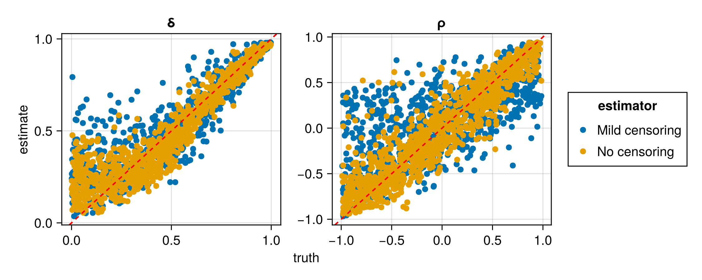
Here we have trained two separate neural estimators to handle two different censoring threshold vectors. However, one could train a single neural estimator that caters for a range of censoring thresholds, c, by allowing it to vary with the data samples and using it as an input to the neural network. In the next section, we illustrate this in the context of peaks-over-threshold modelling, whereby a single censoring threshold is defined to be the marginal -quantile of the data, and we amortise the estimator with respect to the probability level . In a peaks-over-threshold setting, variation in the censoring thresholds can be created by placing a prior on , which induces a prior on c.

Peaks-over-threshold censoring

Richards et al. (2024) discuss neural Bayes estimation from censored data in the context of peaks-over-threshold extremal dependence modelling, where deliberate censoring of data is imposed to reduce estimation bias in the presence of marginally non-extreme events. In these settings, data are treated as censored if they do not exceed their corresponding marginal -quantile, for   close to one.

Peaks-over-threshold censoring, with fixed, can be easily implemented using the General censoring framework by setting the censoring threshold equal to the -th quantile of the data . Further, Richards et al. (2024) show that one can amortise a neural estimator with respect to the choice of by treating it as an input to the neural network.

Below, we sample a fixed set of parameter-data pairs for training the neural network.

# Sampling values of τ to use during training 
function sampleτ(K)
	τ = rand(Uniform(0.0, 0.9), 1, K) 
end

# Adapt the censored data simulation to allow for τ as an input
function simulatecensored(θ, τ, m; kwargs...) 
    Z = simulate(θ, m)
	K = size(θ, 2)
	UW = Folds.map(1:K) do k
        Zₖ = Z[k]
        τₖ = τ[k]
        cₖ = τₖ # data are on uniform margins: censoring threshold equals τ
        mapslices(Z -> censorandaugment(Z; c = cₖ, kwargs...), Zₖ, dims = 1)
	end
end

# Generate the data used for training and validation
K = 50000  # number of training samples
m = 500    # number of replicates in each data set
θ_train  = sample(K)
θ_val    = sample(K ÷ 5)
τ_train  = sampleτ(K)
τ_val    = sampleτ(K ÷ 5)
UW_train = simulatecensored(θ_train, τ_train, m)
UW_val   = simulatecensored(θ_val, τ_val, m)

In this example, the probability level can be incorporated as an input to the neural network by treating it as an input to the outer neural network of the DeepSet architecture. To do this, we increase the input dimension of the outer network by one, and then combine the data and as a tuple (see DeepSet for details).

# Construct neural network based on DeepSet architecture
ψ = Chain(Dense(n * 2, w, relu),Dense(w, w, relu))    
ϕ = Chain(Dense(w + 1, w, relu), final_layer)
network = DeepSet(ψ, ϕ)

# Initialise the estimator
estimator = PointEstimator(network)

# Train the estimator
estimator = train(estimator, θ_train, θ_val, (UW_train, τ_train), (UW_val, τ_val))

Our trained estimator can now be used for any value of within the range used during training ( ). Since the estimator is amortised with respect to , there is no need to retrain it for different degrees of censoring.

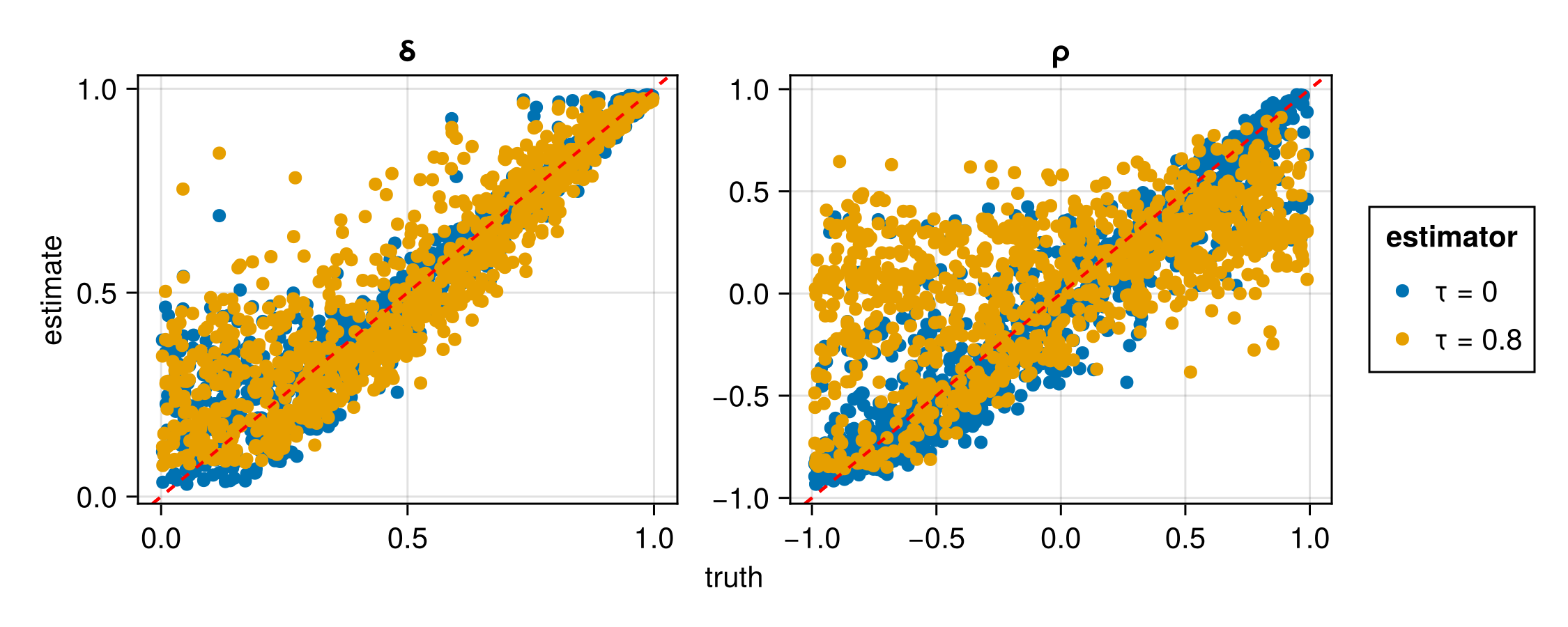
Below, we assess the estimator for different values of . As expected, RMSE increases with (larger corresponds to more censoring).

# Test parameters
θ_test = sample(1000)

# Assessment with τ fixed to 0 (no censoring)
τ_test1  = fill(0.0, 1000)'
UW_test1 = simulatecensored(θ_test, τ_test1, m)
assessment1 = assess(estimator, θ_test, (UW_test1, τ_test1), parameter_names = ["ρ", "δ"], estimator_name = "τ = 0")   

# Assessment with τ fixed to 0.8
τ_test2  = fill(0.8, 1000)'
UW_test2 = simulatecensored(θ_test, τ_test2, m)
assessment2 = assess(estimator, θ_test, (UW_test2, τ_test2), parameter_names = ["ρ", "δ"], estimator_name = "τ = 0.8")   

# Compare results between the two censoring probability levels
assessment = merge(assessment1, assessment2)
rmse(assessment)
plot(assessment)

Estimator	Parameter	RMSE
τ = 0	ρ	0.241780
τ = 0	δ	0.096779
τ = 0.80	ρ	0.476348
τ = 0.80	δ	0.124913